When analyzing data in Excel at times it is necessary to pull data from another data source based on more than one column. In this case you can use the MATCH function in an array formula. Just so you understand the general idea of an array, it is a collection of values. The match function is generally used to find a value in an array. Knowing this, we will use this Excel file to show how to engineer a multi-column VLOOKUP in a few simple steps.

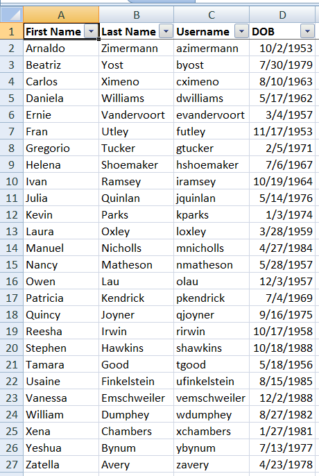
Above is a screenshot of the data in the Source Data tab. On our Lookups tab I started off with just the first names and last names of some users. In order to pull the corresponding usernames and DOBs (dates of birth) I did the following:
-
Setup a column indicating where the matching data was found by using the following array formula:
{=MATCH(1,('Source Data'!$A$2:$A$27=$A1)*('Source Data'!$B$2:$B$27=$B1),0)}- It is important to note that even though the formula is surrounded by curly braces, those are put there by Excel (NOT MANUALLY) when executing the formula by using the
CTRL+SHIFT+ENTERkey combination. - The first parameter (
1) indicates the value being searched for in the second parameter. -
The second parameter is an array which remains such only because of the
CTRL+SHIFT+ENTERkey combination used to finalize the formula.- That will produce an array of 0s and 1s which are coerced into the numbers because of the multiplication operation.
- If there was only one column checked and the multiplication were taken out, the array will be full of
TRUEs andFALSEs. For example the formula=TRUE*TRUEresults in1whileTRUE*FALSEresults in0.
- The third parameter
0indicates that the first parameter must match be an exact match of one of the items in the array (second parameter). - The value returned will be the position (start at
1) of the value in the array if found. If not found an N/A error will be returned.
- It is important to note that even though the formula is surrounded by curly braces, those are put there by Excel (NOT MANUALLY) when executing the formula by using the
-
Setup a new column which references the matching row column to pull the corresponding username if a matching row was found. If the row wasn’t found show the cell as empty:
=IF(ISNA($C2),"",INDEX('Source Data'!$C$2:$C$27,$C2)) -
Setup a new column which references the matching row column to pull the corresponding DOB if a matching row was found. Format the date using the
YYYY-MM-DDformat. If the row wasn’t found show the cell as empty:
=IF(ISNA($C2),"",TEXT(INDEX('Source Data'!$D$2:$D$27,$C2),"YYYY-MM-DD"))
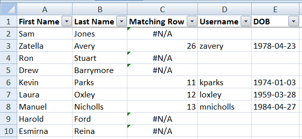
After doing the above three steps in row 2 of the Lookups sheet and copying the formulas down, the final result was this:

If I were to clean this up a bit more I might hide column C of the Lookups tab, but other than that there really isn’t much else you need to do. I know this may still seem a bit mysterious, but with practice you will begin to understand array formulas better and perhaps write other useful array formulas to get the job done. For all of you who came to figure out how to do a multi-criteria lookup, I hoped it helped but if not, comment on what needs clarifying and I will do my best to help. 😎


